DeepComplete

Generative Adversarial Autoencoders for Multiple Imputation

Luna Bellitto, Will de Melo, Erika Garza-Elorduy, Emily Han, Umberto Mignozzetti, and Asad Tariq (UCSD)

Introduction

• Missing data has been a persistent issue in empirical political science.

• It leads to biased results and compromises the validity of analyses (King et al., 2001; Zhang, 2015; Lall 2016, 2017; Stavseth, 2019; Lall and Robinson, 2022).

• Traditional multiple imputation methods:

  1. Fail to capture non-linear data representations.
  2. Often operate under parametric assumptions.
  3. Sometimes use MCMC, which may take considerably longer to estimate (Kropco et al. 2014).

• Recently, Deep Learning advances have provided easy-to-use and fast new methods for multiple imputation (Gondara and Wang 2018; Ma et al. 2020; Lall and Robinson, 2022; Lall and Robinson, 2023)

Introduction

• In this project, we present a new methodology for performing multiple imputations: DeepComplete

• DeepComplete uses adversarial autoencoders (Makhzani et al., 2014) for multiple imputations, attacking the encoder and the full generative process.

• Key Features:

  1. Combines autoencoders with adversarial networks to map original data into a low-dimensional latent space ($l = 2$).
  2. Uses a Wasserstein GAN discriminator (Guljarani et al. 2017) to refine and stabilize the latent space, helping a robust data reconstruction.
  3. Perform completions not only using denoising, but also actively engaging with the latent space structure (Convex Hull completion).

Introduction

• To evaluate DeepComplete, we used a 3631 sample from the 2020 ANES survey, with 27 variables and the MNIST hand written digits data.

  • Since the MNIST data is still running, we will present only the ANES results in here.

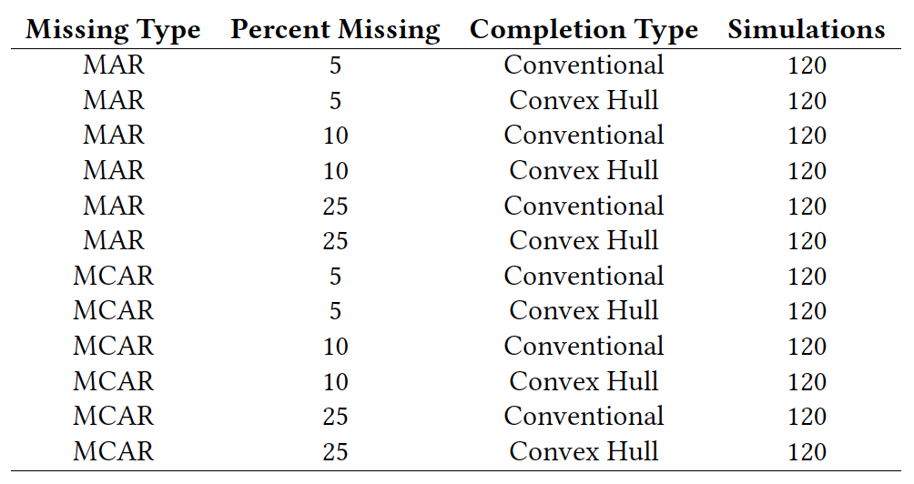
• We created 720 datasets varying the amont of missingness, the type of missingness (MAR x MCAR).

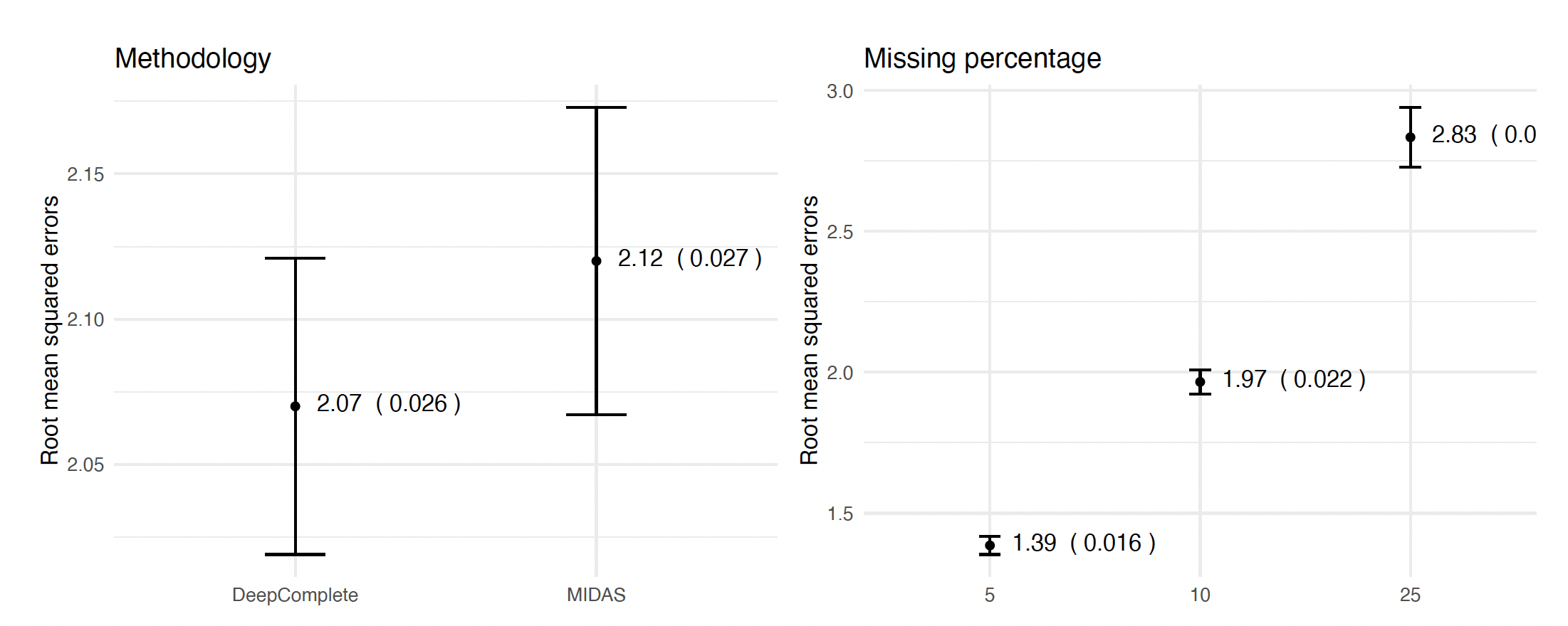
• We show that DeepComplete:

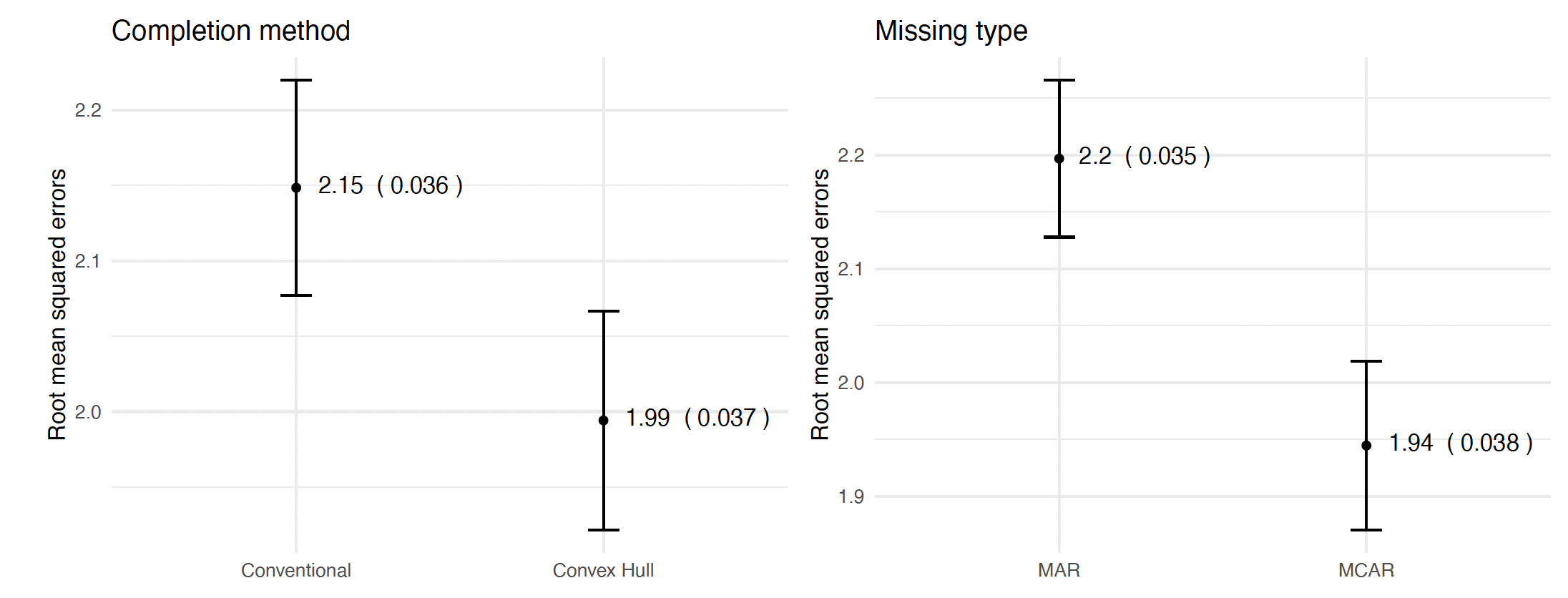
  1. Presents an MSE reconstruction of 2.07 (SE=0.026), which is slightly better than MIDAS (2.12, SE=0.027).
  2. Using the convex hull multiple imputation approach has a smaller MSE (1.99, SE=0.037) than conventional sampling (2.15, SE=0.036).
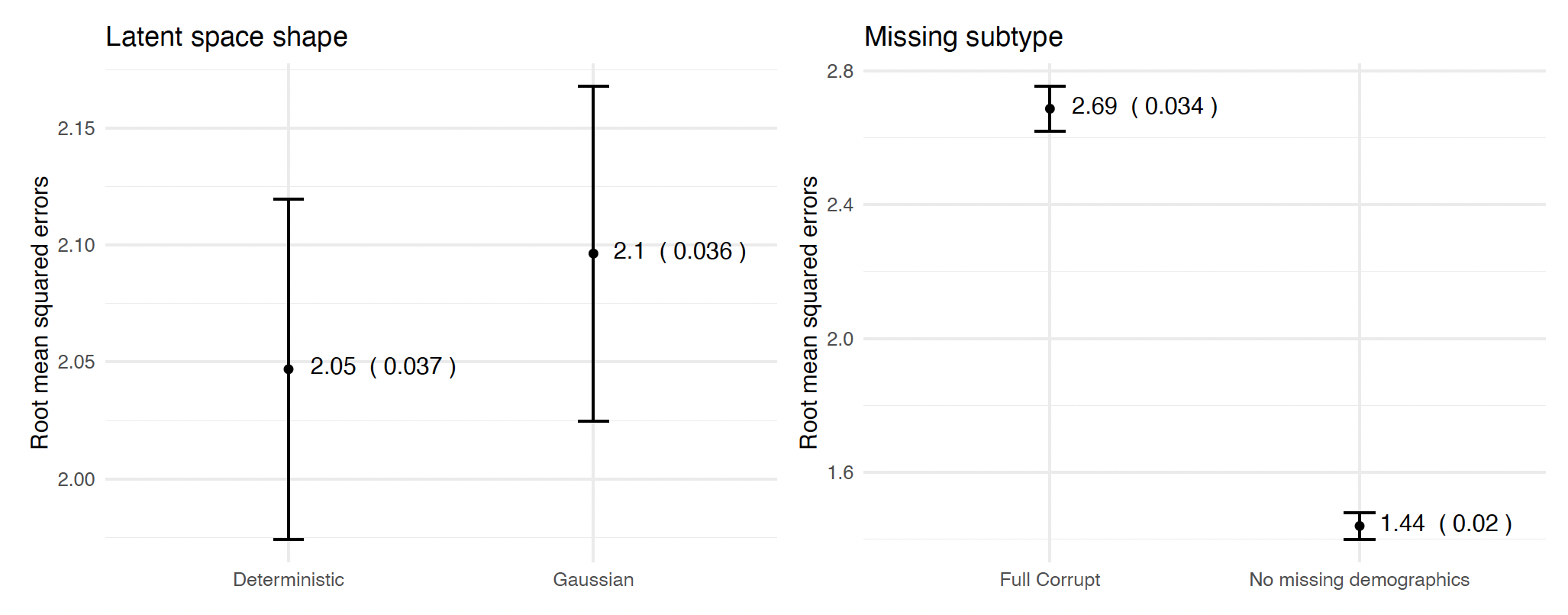
  3. Deterministic latent structures perform slightly better (2.05, SE=0.037) than Gaussian latent structures (2.10, SE=0.037).
  4. (expected) Imputations on MCAR perform better (1.94, SE=0.037) than MAR (2.20, SE=0.035)
  5. (expected) Lower the missing amounts result in better imputation quality.

• But DeepComplete still performs 1.7 times slowlier than MIDAS, most likely because it fits two neural networks at each run.

Autoencoders

• Autoencoders were proposed by Hinton and Salakhutdinov (2006) as a type of "non-linear" PCA, using neural networks.

• Since then, many types of Autoencoders have been proposed, for applications such as anomaly detection, data compressing, and data reconstruction.

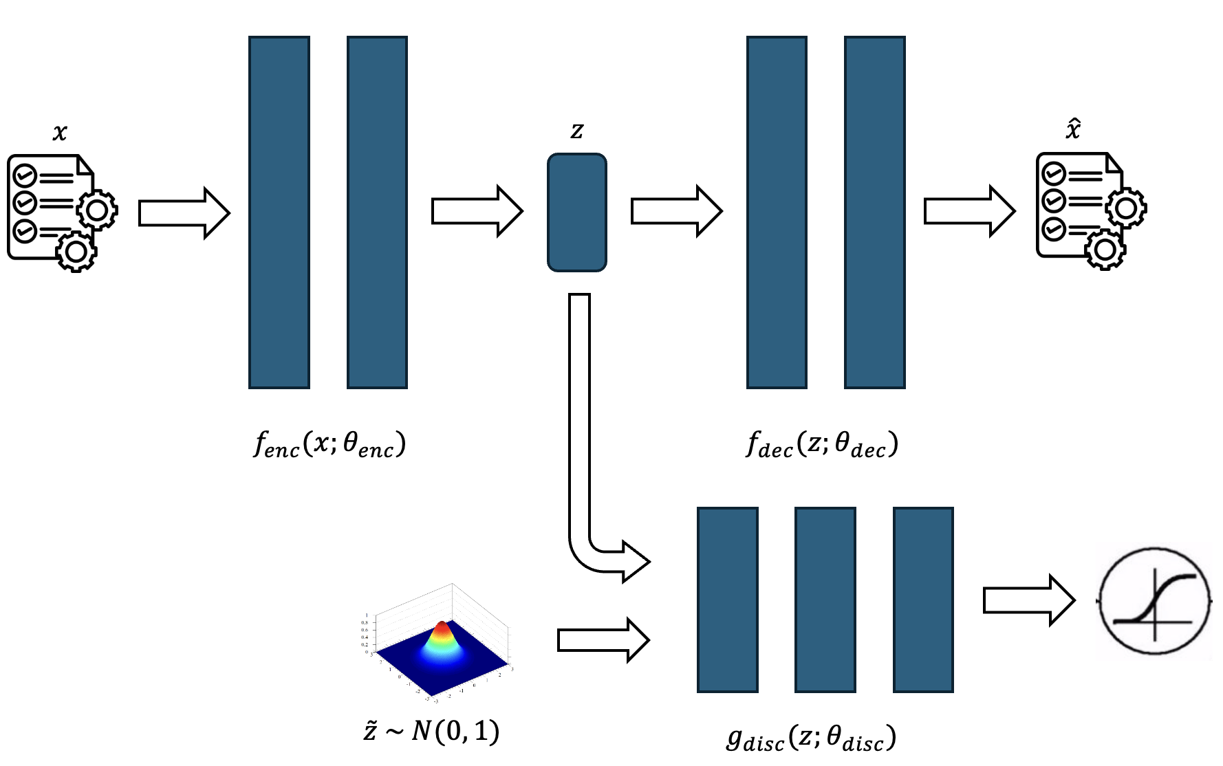
• The basic architecture of an autoencoder:

  1. Receives $k$-dimensional data ($x \in \mathbb{R}^k$) and maps it into an $f_{\text{enc}}: \mathbb{R}^k \times \mathbb{R}^n \rightarrow \mathbb{R}^l$, encoding it into a $l$-dimensional manifold ($z \in \mathbb{R}^l$).

  2. Take the $l$-dimensional latent representation ($z \in \mathbb{R}^l$) and maps back into the original space by passing a transformation $f_{\text{dec}}: \mathbb{R}^l \times \mathbb{R}^m \rightarrow \mathbb{R}^k$.

• Any functional forms $(f_{\text{enc}}, f_{\text{dec}})$ may be used, and here we use neural networks, since they have powerful properties when it comes to detect high non-linearities in the data.

Autoencoders

• However, encoding data in way has a few disadvantages. and to fix some of these problems, regularizations have been proposed so that the latent space is reshaped in a way that stabilizes training.

• Among the three most important regularizations:

  1. Variational autoencoders: Imposing a KL divergence penalty whenever the latent space deviates from a given parametric distribution (Kingma and Welling, 2013)
  2. Moment-matching networks: Ensures that as many moments of the latent distribution match pre-determined values (Li et al., 2015)
  3. Adversarial attacks: Way to regularize the space by creating a zero-sum game between two neural networks (Makhzani et al. 2015)

• A fourth regularization, most common in corrupt data applications is Denoising (Vincent et al. 2010).

  • It consists in corrupt fractions of the input and use the uncorrupted data as benchmarking in training.

Autoencoders

• In DeepComplete, we use Denoising + Adversarial attacks.

• Denoising:

  • After finish training the autoencoder, I reduce original learning rate (0.001) by a factor of one thousand (0.000001)
  • Propose a corrupt schedule of (5%, 10%, 15%, and 20%).
  • Refit the algorithm

• The denoising process have a two-fold benefit:

  1. Avoids identity-mapping (overfitting)
  2. Improves the stability of the reconstructed space.

Adversarial Autoencoders

• Adversarial Autoencoders:

  • Adversarial Networks are neural networks that are trained separately, but with loss functions linked.

  • In DeepComplete, the adversary (called discriminator) is 1-Lipschitz function $g_\text{disc}: \mathbb{R}^l \times \mathbb{R}^p \rightarrow [-\infty, \infty]$ that receives data from the encoder and from a given distribution, and scores it.

  • We then tie these networks together:

    1. Training the loss function of the discriminator to maximize accuracy (getting better in telling if a set of points came from the preset distribution)

    2. Training the loss function of the encoder to try to fool the discriminator.

• The equilibrium of this game makes the encoder very skilled in producing results close by the preset distribution.

• This has regularizing effects that go beyond mode selection, improving the shape of the latent space and its contiguity (Makhzani et al. 2015)

Adversarial Autoencoders

The full DeepComplete setup is as follows:

Adversarial Autoencoders for Multiple Imputation

• But most applications of autoencoders consider the latent space as a step in the process.

• They rarely engage with it, unless for penalizing them based on a given distribution, with the objective of improving algorithm convergence.

• The latent space are basically considered to be blobs of information.

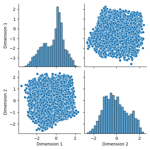
Adversarial Autoencoders for Multiple Imputation

The "blob assumption" may be correct for some variables:

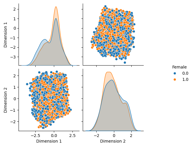
Adversarial Autoencoders for Multiple Imputation

But not for others:

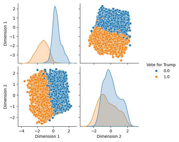
Therefore, we can use information from the latent space to improve the imputation quality.

Adversarial Autoencoders for Multiple Imputation

• In this project, we created a method to engage with the latent space, using proximate values of an intended generated observation, to improve the outcome of the multiple imputation.

• It consists in:

  1. Select $k$ observations close to the original data (disconsidering the missing values)
  2. Find the latent representation of these $k$ values
  3. Compute the Convex-Hull formed by these $k$ values
  4. Sample a reconstruction (the data to impute) from this Convex-Hull.

We call this procedure Convex Hull imputation.

Simulations

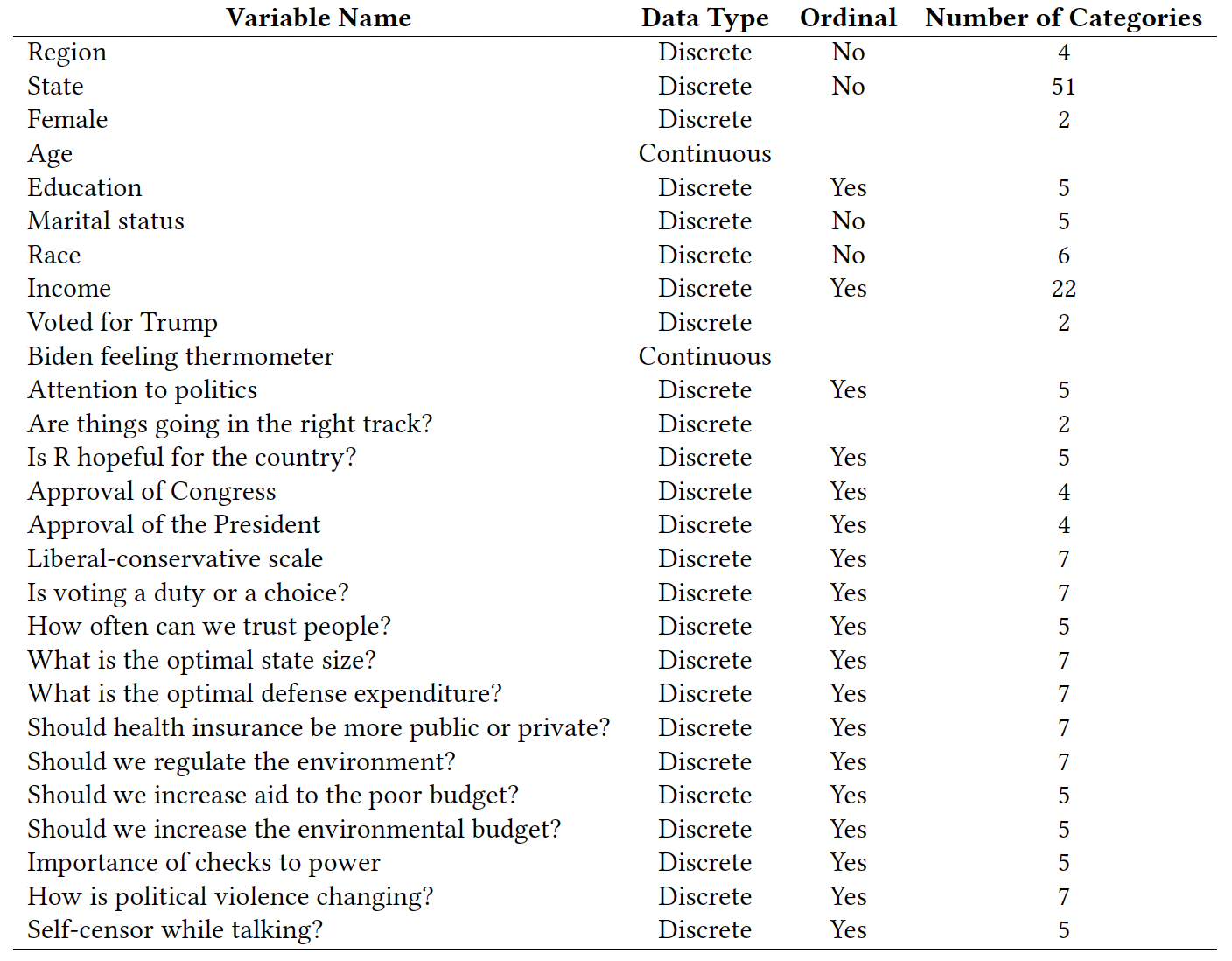
We perform simulations using the 2020 ANES dataset. We selected complete observations for 3631 values and 27 variables:

Simulations

We perform the following simulations:

Results

Results

Results

Conclusion

• DeepComplete:

  • Introduces an adversarial autoencoder technique for multiple imputations.
  • Combines autoencoders with adversarial networks for robust data reconstruction.
  • Utilizes convex hull sampling to improve imputation accuracy.

• Performance:

  • Slightly better imputation performance compared to traditional methods like MIDAS (but slowlier).
  • Effective in handling both missing completely at random (MCAR) and missing at random (MAR) patterns.

• Contributions:

  • Provides a flexible and effective solution for handling missing data in political science datasets.
  • Enhances data completeness and analytical robustness.

• Next Steps:

  • Get the MNIST to work and find a text example.
  • Build a method to evaluate the quality of the imputation using the latent space.